SMV2rho: Tutorial 5

In this tutorial we will see how we can include temperature dependence within the density conversion scheme. Note that this is only pssible with the SMV2rho 'stephenson' scheme because the 'brocher' approach is explicitly not a temperature or pressure dependent approach and so we do not recommend including this dependency with this scheme.

Secondly, we will explore the option to set the uppermost layer of the crust to have a constant density. This option allows us to exclude the portion of the crust that experiences an exponential velocity drop-off.

# import modules
import numpy as np
from SMV2rho import plotting as smplt
from SMV2rho import density_functions as smd
from SMV2rho import constants as c
from SMV2rho import temperature_dependence as td

Intel MKL WARNING: Support of Intel(R) Streaming SIMD Extensions 4.2 (Intel(R) SSE4.2) enabled only processors has been deprecated. Intel oneAPI Math Kernel Library 2025.0 will require Intel(R) Advanced Vector Extensions (Intel(R) AVX) instructions.
Intel MKL WARNING: Support of Intel(R) Streaming SIMD Extensions 4.2 (Intel(R) SSE4.2) enabled only processors has been deprecated. Intel oneAPI Math Kernel Library 2025.0 will require Intel(R) Advanced Vector Extensions (Intel(R) AVX) instructions.

Class approach

Again we will first go through this procedure step-by-step so that we can query the outputs.

Load file

Let’s define the velocity profile that we are interested in converting, initialise the Convert and Constants classes and read in the profile data file.

# path to test velocity file
#  - this file comes with the distribution so there is no need to change this path
vp_file = "../TEST_DATA/EUROPE/Vp/RECEIVER_FUNCTION/DATA/M19_AQU_Vp.dat"

# create the constants object.
constants = c.Constants()

Creating the geotherm object

For a temperature-dependent parametrisation, we must provide an estimate of the temperature structure at depth. To do so, we need to parameterise the geothermal gradient. SMV2rho incorporates a number of geothermal parametrisations, with hopefully more to come.

To create the geotherm object, we frst instantiate the Geotherm class within the temperature_dependence module. At this stage, we can select a number of different parametrisations for the geotherm, including a simple, linear geotherm or various different approches that solve the 1D heat equation with internal heat production for various boundary conditions. Which geotherm you pick will depend on the constraints present (e.g. do you have a constraint on Moho temperature vs Moho heat flux etc?). the default option is 'linear', i.e. a simple geotherm that is linear and defined by surface and basal temperature. Please see the documentation for the Geotherm class and the GeothermConstants dataclass for more information.

Note that for the Geotherm class, depths, including crustal thickness, depth below surface, and the depth range over which geothermal heat production decays away must be given in positive kilometres and density must be given in g/cm3. This is consistent with other parameters elsewhere in SMV2rho, although we acknowledge that using SI units would be preferable in some circumstances.

below we will generate three geotherms using different methods. Note all will use default values stored in the GeothermConstants data class, which can all be set manually when creating the geotherm object. For example geotherm = td.Geotherm(geotherm_type = "linear", tc = 30, k = 3.0, H0 = 7.5e-10 ...) to select manual options.

# create a depth array for plotting
z = np.linspace(0, 40, 100)

# create a linear geotherm object providing a crustal thickness (in m)
geotherm1 = td.Geotherm(tc = 30)
# calculate the geotherm by calling the geotherm class
T_arr1 = geotherm1(z)

# create a geotherm object that depends on heat flux at surface and moho
# note this does not require a crustal thickness argument
geotherm2 = td.Geotherm(geotherm_type = 'single_layer_flux_difference')
T_arr2 = geotherm2(z)

# create a geotherm object that depends on temperature at the surface and at the moho
geotherm3 = td.Geotherm(geotherm_type = 'single_layer_temperature_difference', tc = 30)
T_arr3 = geotherm3(z)

#### PLOTTING ####

# data1, data2 and data3 -- list of dictionaries for each panel for each data series.
data1 = [{'x': T_arr1, 'y':-z}]
data2 = [{'x':  T_arr2, 'y':-z}]
data3 = [{'x':  T_arr2, 'y': -z}]

titles = ['linear', 'q difference', 'T difference']
xlabels = ['T', 'T', 'T']
ylabels = ['Depth (km)', 'Depth (km)', 'Depth (km)']

# Call the plot_panels function
smplt.plot_panels(
    [data1, data2, data3],
    plot_type='line',
    cmap=None, titles=titles,
    xlabels=xlabels,
    ylabels=ylabels,
    z_values=None,
    figure_scale=0.7,
    save_path=None)

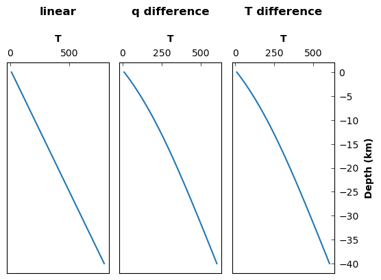
Let’s create the geotherm object for the profile that we will be using. We will use a single-layer model with internal heat generation defined by surface and basal heat flow using

\(T(z) = T_0 + \frac{q_m z}{k} + \frac{(q_0 - q_m) h_r}{k} \left[ 1 - \exp \left( \frac{-z}{h_r} \right) \right]\),

where \(T_0 = 10\)~:nbsphinx-math:textdegree `C is the temperature at the surface, :math:`q_0 = 59 pm 14 mW m $^{-2} $ and \(q_m = 30 \pm 10\) mW m \(^{-2}\) are the surface and Moho heat flux, respectively, \(h_r = 10\) km is a characteristic length scale describing the rate of decrease of internal heat production with depth, and \(k = 2.5\) W m \(^{-1}\) K \(^{-1}\) is the thermal conductivity.

geotherm = td.Geotherm(geotherm_type = 'single_layer_flux_difference')

Convert Profile

This time we will set T_dependence = True, which is the default setting so we won’t pass it as an argument here. This option will prompt the program to look for a a material_constants attribute within the constants class instance. At the moment, this object does not exist and so the program will throw an error!

# load a profile into the Convert class
profile = smd.Convert(
    vp_file,
    profile_type = "Vp",
    geotherm = geotherm
    )

# read data
profile.read_data()

# calculate density profile -- note default is the temperature dependence is True!
profile.V_to_density_stephenson(
    constants,
    T_dependence = True
    )

---------------------------------------------------------------------------
ValueError                                Traceback (most recent call last)
Cell In[5], line 12
      9 profile.read_data()
     11 # calculate density profile -- note default is the temperature dependence is True!
---> 12 profile.V_to_density_stephenson(
     13     constants, 
     14     T_dependence = True
     15     )

File ~/Work/SMV2rho/src/SMV2rho/density_functions.py:474, in Convert.V_to_density_stephenson(self, parameters, dz, constant_depth, constant_density, T_dependence, plot)
    439 def V_to_density_stephenson(self, parameters,
    440                             dz=0.1,
    441                             constant_depth = None,
    442                             constant_density = None,
    443                             T_dependence = True,
    444                             plot = False):
    445     """
    446     Convert seismic velocity profiles to density using the Stephenson 
    447     method.
   (...)
    471         None
    472     """
--> 474     check_arguments(T_dependence, constant_depth, constant_density,
    475                         "stephenson", parameters, self.geotherm)
    477     # instantiate convert profile calss
    478     ProfileConvert = V2RhoStephenson(self.data,
    479                                      parameters,
    480                                      self.profile_type,
   (...)
    483                                      T_dependence,
    484                                      self.geotherm)

File ~/Work/SMV2rho/src/SMV2rho/density_functions.py:1379, in check_arguments(T_dependence, constant_depth, constant_density, approach, parameters, geotherm)
   1377 elif isinstance(parameters, c.Constants) is True:
   1378     if parameters.material_constants is None:
-> 1379         raise ValueError("T_dependence is set to True but "
   1380                     "material_constants instance of the Constants "
   1381                     "class has not been set.")
   1383 if not geotherm:
   1384     raise ValueError("Please create a geotherm object using the `Geotherm` "
   1385           "class")

ValueError: T_dependence is set to True but material_constants instance of the Constants class has not been set.

We can now set up the constants object by calling the get_v_constants method as in the last tutorial. This time we will also call the get_material_constants method which will generate the constants for the temperature-dependent part of the conversion.

# call the get_v_constants method asking for Vp constants
constants.get_v_constants('Vp')

# call the get_material_constants method
constants.get_material_constants()

print(constants)

Constants(vp_constants=VpConstants(v0=-0.93521, b=0.00169478, d0=2.55911, dp=-0.00047605, c=1.674065, k=0.01953466, m=-0.0004, v0_unc=None, b_unc=None, d0_unc=None, dp_unc=None, c_unc=None, k_unc=None, m_unc=0.0001), vs_constants=None, material_constants=MaterialConstants(alpha0=1e-05, alpha1=2.9e-08, K=90000000000.0, alpha0_unc=5e-06, alpha1_unc=5e-09, K_unc=20000000000.0))

We can see that the constants object now contains a VpConstants object and a MaterialsConstants object.

Now we can run the conversion again and this time it will work.

Note, as with the previous tutorial, running this function may result in an integration warning. This warning can be safely ignored and is generated because the velocity and density profile functions \(V_P(z)\) and \(\rho (z)\) contain discontinuities.

constants.material_constants

MaterialConstants(alpha0=1e-05, alpha1=2.9e-08, K=90000000000.0, alpha0_unc=5e-06, alpha1_unc=5e-09, K_unc=20000000000.0)

# calculate density profile -- note default is the temperature dependence is True!
profile.V_to_density_stephenson(constants, T_dependence = True)

profile.data.keys()

/Users/eart0518/Work/SMV2rho/src/SMV2rho/density_functions.py:1698: IntegrationWarning: The maximum number of subdivisions (50) has been achieved.
  If increasing the limit yields no improvement it is advised to analyze
  the integrand in order to determine the difficulties.  If the position of a
  local difficulty can be determined (singularity, discontinuity) one will
  probably gain from splitting up the interval and calling the integrator
  on the subranges.  Perhaps a special-purpose integrator should be used.
  int_val = integrate.quad(interp_profile, bins_low_res[e],

dict_keys(['station', 'Vp_file', 'region', 'moho', 'location', 'av_Vp', 'Vp', 'type', 'method', 'geotherm', 'rho', 'av_rho', 'rho_hi_res', 'Vp_hi_res', 'p', 'T'])

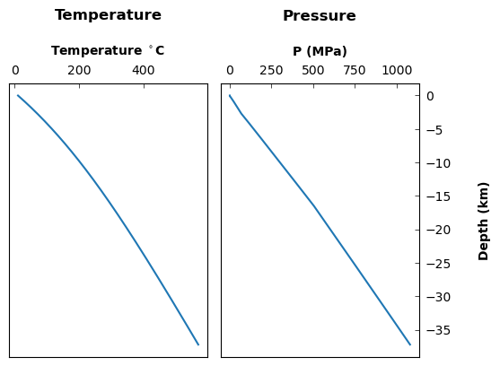
Outputs and plotting

We can now explore the outputs. We can already see that we now have a 'T' key within the output dictionary. This temperature profile is generated using a constant moho and surface heat flux with heat production concentrated within the upper 10 km. It is possible to edit the parametrisation of the geotherm within the temperature_dependence and density_functions modules.

# Define plot settings
plot_type = 'line'
titles = ['Temperature', 'Pressure']
xlabels = [r'Temperature $^\circ$C', 'P (MPa)']
ylabels = ['Depth (km)', 'Depth (km)']

# data1, data2 and data3 -- list of dictionaries for each panel for each data series.
data1 = [{'x': profile.data["T"][:,1], 'y': profile.data["T"][:,0]}]
data2 = [{'x': profile.data["p"][:,1], 'y': profile.data["p"][:,0]}]

# Call the plot_panels function
smplt.plot_panels(
    [data1, data2],
    plot_type=plot_type,
    cmap=None, titles=titles,
    xlabels=xlabels,
    ylabels=ylabels,
    z_values=None,
    figure_scale=0.7,
    save_path=None)

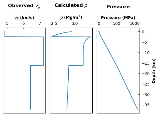
Now let’s plot up the velocity and density curves

# Define plot settings
plot_type = 'line'
titles = [r'Observed ${V_p}$', r'Calculated $\rho$']
xlabels = [r'${V_P}$ (km/s)', r'$\rho$ (Mg/m${^3}$)']
ylabels = ['Depth (km)', 'Depth (km)']

# data1, data2 and data3 -- list of dictionaries for each panel for each data series.
data1 = [{'x': profile.data["Vp_hi_res"][:,1], 'y': profile.data["Vp_hi_res"][:,0]}]
data2 = [{'x': profile.data["rho_hi_res"][:,1], 'y': profile.data["rho_hi_res"][:,0]}]

# Call the plot_panels function
smplt.plot_panels(
    [data1, data2],
    plot_type=plot_type,
    cmap=None, titles=titles,
    xlabels=xlabels,
    ylabels=ylabels,
    z_values=None,
    figure_scale=0.7,
    save_path=None)

Function approach

Again, it is possible, by using the options in the convert_V_profile function, to convert this velocity profile using a function rather than step-by-step using the class objects.

# call density conversion function
# note that using profile_type="Vs" first calls a function to convert to Vp
# as is required by Brocher's (2005) approach.
profile_stephenson = smd.convert_V_profile(
    vp_file,
    profile_type="Vp",
    approach="stephenson",
    print_working_file = True,
    parameters = constants,
    T_dependence = True,
    geotherm = geotherm
    )

working on ../TEST_DATA/EUROPE/Vp/RECEIVER_FUNCTION/DATA/M19_AQU_Vp.dat

# data1, data2 and data3 -- list of dictionaries for each panel for each data series.
data1 = [{'x': profile_stephenson["Vp_hi_res"][:,1], 'y': profile_stephenson["Vp_hi_res"][:,0]}]
data2 = [{'x': profile_stephenson["rho_hi_res"][:,1], 'y': profile_stephenson["rho_hi_res"][:,0]}]
data3 = [{'x': profile_stephenson["p"][:,1], 'y': profile_stephenson["p"][:,0]}]

titles = [r'Observed ${V_p}$', r'Calculated $\rho$', 'Pressure']
xlabels = [r'${V_P}$ (km/s)', r'$\rho$ (Mg/m${^3}$)', 'Pressure (MPa)']
ylabels = ['Depth (km)', 'Depth (km)', 'Depth (km)']

# Call the plot_panels function
smplt.plot_panels(
    [data1, data2, data3],
    plot_type=plot_type,
    cmap=None, titles=titles,
    xlabels=xlabels,
    ylabels=ylabels,
    z_values=None,
    figure_scale=0.7,
    save_path=None)

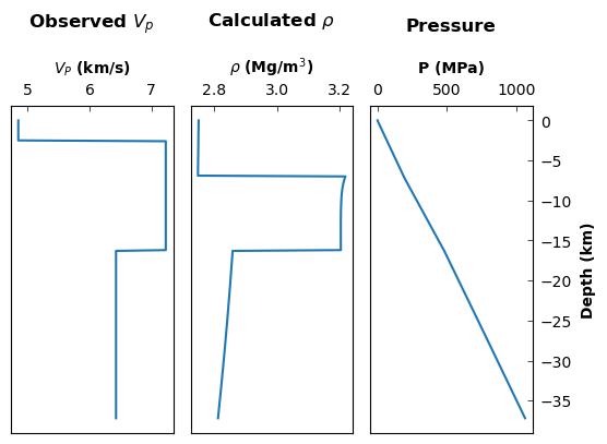
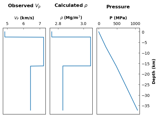
Excluding the uppermost \(x\) km

We can exclude the uppermost \(x\) km from the density conversion, setting it to a constant value in order to avoid mismatches between exponential drop-off in the density conversion scheme that may or may not be present in the true velocity profile. This effect can be seen in the above example, where the layers are relatively coarse, and so an exponential veocity dropoff is imposed upon a layer of constant velocity.

To avoid this mismatch, we can set the constant_density and constant_depth parameters. Both of these parameters must be set together.

# calculate density profile -- note default is that temperature dependence is True!
profile.V_to_density_stephenson(
    constants,
    T_dependence = True,
    constant_density = 2.75,
    constant_depth = 7)

Now we can plot the 'rho_hi_res' array and see that the uppermost 7 km have been set to a density of 2.75 Mg/m3. Note that if we are using the temperature_dependence = True option, then we are setting \(\rho_\circ\) to constant, but this density value will still be subject to thermal expansion and compression.

# Define plot settings
plot_type = 'line'
titles = [r'Observed ${V_p}$', r'Calculated $\rho$', 'Pressure']
xlabels = [r'${V_P}$ (km/s)', r'$\rho$ (Mg/m${^3}$)', 'P (MPa)']
ylabels = ['Depth (km)', 'Depth (km)', 'Depth (km)']

# data1, data2 and data3 -- list of dictionaries for each panel for each data series.
data1 = [{'x': profile.data["Vp_hi_res"][:,1], 'y': profile.data["Vp_hi_res"][:,0]}]
data2 = [{'x': profile.data["rho_hi_res"][:,1], 'y': profile.data["rho_hi_res"][:,0]}]
data3 = [{'x': profile.data["p"][:,1], 'y': profile.data["p"][:,0]}]

# Call the plot_panels function
smplt.plot_panels(
    [data1, data2, data3],
    plot_type=plot_type,
    cmap=None, titles=titles,
    xlabels=xlabels,
    ylabels=ylabels,
    z_values=None,
    figure_scale=0.7,
    save_path=None)

And now we can plot the 'rho' array to see what the profile looks like after averaging into the same layers as contained in the input velocity profile.

# Define plot settings
plot_type = 'line'
titles = [r'Observed ${V_p}$', r'Calculated $\rho$', 'Pressure']
xlabels = [r'${V_P}$ (km/s)', r'$\rho$ (Mg/m${^3}$)', 'P (MPa)']
ylabels = ['Depth (km)', 'Depth (km)', 'Depth (km)']

# data1, data2 and data3 -- list of dictionaries for each panel for each data series.
data1 = [{'x': profile.data["Vp_hi_res"][:,1], 'y': profile.data["Vp_hi_res"][:,0]}]
data2 = [{'x': profile.data["rho"][:,1], 'y': profile.data["rho"][:,0]}]
data3 = [{'x': profile.data["p"][:,1], 'y': profile.data["p"][:,0]}]

# Call the plot_panels function
smplt.plot_panels(
    [data1, data2, data3],
    plot_type=plot_type,
    cmap=None, titles=titles,
    xlabels=xlabels,
    ylabels=ylabels,
    z_values=None,
    figure_scale=0.7,
    save_path=None)

Exploring different parameter values

We can explore the effects of using different values of various parameters. Let’s explore the rfesult if we use a different value for \(m\), the linear dependence of velocity on \(T\).

constants1 = c.Constants()

# call the get_v_constants method asking for Vp constants
constants1.get_v_constants('Vp', m = -0.1e-4)

# call the get_material_constants method
constants1.get_material_constants()

# call density conversion function
# note that using profile_type="Vs" first calls a function to convert to Vp
# as is required by Brocher's (2005) approach.
profile1_stephenson = smd.convert_V_profile(
    vp_file,
    profile_type="Vp",
    approach="stephenson",
    print_working_file = True,
    parameters = constants1,
    T_dependence = True,
    geotherm = geotherm)

# plot density profiles
data_m_test = [
    {'x': profile1_stephenson["rho"][:,1],
     'y': profile1_stephenson["rho"][:,0],
     'label':'small m'},
     {'x': profile_stephenson["rho"][:,1],
      'y': profile_stephenson["rho"][:,0],
      'label':'larger m'}
      ]

# Call the plot_panels function
smplt.plot_panels([data_m_test], plot_type='line',
            cmap=None, titles=None,
            xlabels=[r'$\rho$ (Mg/m${^3}$)'], ylabels=['Depth (km)'],
            z_values=None, figure_scale=0.7,
            save_path=None)

working on ../TEST_DATA/EUROPE/Vp/RECEIVER_FUNCTION/DATA/M19_AQU_Vp.dat

/Users/eart0518/Work/SMV2rho/src/SMV2rho/density_functions.py:1698: IntegrationWarning: The maximum number of subdivisions (50) has been achieved.
  If increasing the limit yields no improvement it is advised to analyze
  the integrand in order to determine the difficulties.  If the position of a
  local difficulty can be determined (singularity, discontinuity) one will
  probably gain from splitting up the interval and calling the integrator
  on the subranges.  Perhaps a special-purpose integrator should be used.
  int_val = integrate.quad(interp_profile, bins_low_res[e],

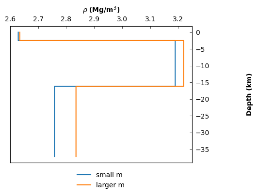
So we can clearly see that picking a larger value of \(m\), or \(\frac{\partial V_P}{\partial T}_P\) leads to an increase in our density estimate.

Summary

We have now included temperature dependence within the density conversion scheme. We have explored how to create an instance of the Constants class including a material_constants object and we have explored how to set the uppermost \(x\) km to a constant value to mitigate cases where the expected exponential dropoff in velocity is not reflected in the velocity profile. We also played with changing certain parameters to explore the effect that they have on velocity profiles.